
🌿Lotka-Volterra Calculator
| Step | Description | Substituted Formula | Result |
|---|
Table of Contents
✍️ Author & Academic Authority: Dr. Nitish Kr. Bharadwaj
📘 Qualifications: B.Sc., B.Ed., M.Sc., Ph.D. (Biochemistry), MBA (Financial Management)
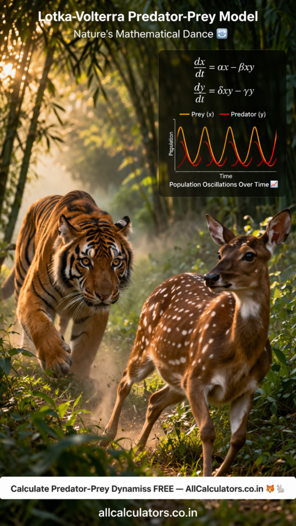
🦊🐇 Lotka Volterra Calculator
Solve Predator-Prey Population Dynamics Instantly Online 🌿📊
Nature is not a static painting 🖼️ — it is a living, breathing, constantly oscillating system where life feeds upon life, populations boom and crash, and species are locked in an eternal dance of survival 🌍. At the mathematical heart of this living drama sits one of science’s most elegant and powerful frameworks: the Lotka-Volterra equations 🧮. Whether you are a biology student grappling with differential equations 📚, an ecology researcher modeling wildlife populations 🦁, or simply a curious mind trying to understand why rabbit and fox populations rise and fall together in mysterious cycles 🐇🦊 — our free online Lotka-Volterra Calculator at AllCalculators.co.in is your ultimate companion. Solve, simulate, and explore predator-prey dynamics instantly, without writing a single line of code! ⚡
📜 What are the Lotka-Volterra Equations? A Journey Through History
The Lotka-Volterra predator-prey model carries the names of two brilliant scientific minds who, working independently on opposite sides of the Atlantic, arrived at the same extraordinary mathematical insight. 🇺🇸 Alfred James Lotka (1880–1949), an American mathematician and physical chemist, first formulated the equations in 1910 while studying autocatalytic chemical reactions, and later in 1920 extended them to describe biological population dynamics in organic systems. 🇮🇹 Vito Volterra (1860–1940), an Italian mathematician and physicist, published an identical set of equations in 1926, motivated by a fascinating real-world puzzle: his son-in-law, the marine biologist Umberto D’Ancona, had noticed that during World War I (1914–1918), when fishing activity in the Adriatic Sea was drastically reduced, the proportion of predatory fish in catches actually increased rather than decreased 🐟. Volterra’s mathematical model perfectly explained this counterintuitive observation, cementing the Lotka-Volterra equations as one of the founding pillars of mathematical ecology and population biology 🏛️.
🔬 Understanding the Lotka-Volterra Model: Core Concept
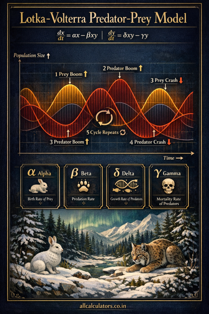
At its essence, the Lotka-Volterra model describes a two-species ecosystem where one species (the prey 🐇) is consumed by another (the predator 🦊). The populations of both species change over time in a beautifully coupled, cyclic fashion — when prey are abundant, predators thrive; when predators multiply, prey numbers crash; when prey become scarce, predators starve and decline; and finally, with predator pressure lifted, the prey recover — and the cycle begins again 🔄. This perpetual oscillation is the defining signature of the Lotka-Volterra system, and it has been observed in countless real ecosystems from the famous Canadian lynx and snowshoe hare cycle (documented over 90 years by the Hudson’s Bay Company 🦎) to phytoplankton and zooplankton in ocean systems 🌊.
📐 The Lotka-Volterra Differential Equations Explained
The Lotka-Volterra predator-prey model is expressed as a pair of coupled first-order, nonlinear ordinary differential equations (ODEs):
Prey Population Equation: 🐇 dx/dt = αx − βxy
Predator Population Equation: 🦊 dy/dt = δxy − γy
Where the four Greek parameters represent:
| Parameter | Symbol | Meaning |
|---|---|---|
| 🐇 Prey Growth Rate | α (alpha) | The natural per-capita birth/growth rate of prey in the absence of predators (exponential growth coefficient) |
| ⚔️ Predation Rate | β (beta) | The rate at which predators consume prey per unit of both populations; represents predator-prey encounter frequency |
| 🍖 Predator Conversion Efficiency | δ (delta) | The rate at which consumed prey are converted into new predator births; predator reproduction efficiency |
| 💀 Predator Death Rate | γ (gamma) | The natural per-capita death/decay rate of predators in the absence of prey |
The term αx represents the exponential growth of prey in a predator-free world 🌱. The term βxy is the predation term — it captures the rate at which predators remove prey, proportional to how frequently the two populations “meet.” In the predator equation, δxy represents the growth of the predator population fueled by prey consumption, while γy models the natural die-off of predators in the absence of food 🍂.
🎯 The Equilibrium Point: Where Predator and Prey Find Balance
A critical insight from the Lotka-Volterra model is the coexistence equilibrium point — the theoretical population sizes at which neither species grows nor declines:
🐇 Prey Equilibrium (x) = γ / δ* 🦊 Predator Equilibrium (y) = α / β*
This equilibrium is mathematically a center — meaning populations orbit around it endlessly in closed cycles, never settling to a fixed point. The size and shape of the orbit depends entirely on the initial conditions (starting population sizes), which is one of the model’s key theoretical features and one of its acknowledged limitations in representing real-world ecosystems where random disturbances continually push populations away from their theoretical orbits 🌀.
🧠 Key Assumptions of the Lotka-Volterra Model
Like all models, the Lotka-Volterra system is built upon a set of simplifying assumptions that define its scope and limitations:
- ✅ Unlimited Prey Resources — Prey have access to infinite food and will grow exponentially without predators
- ✅ Predator Dependence on Prey — Predators rely entirely on prey for sustenance; no alternative food source
- ✅ Proportional Predation — The predation rate is directly proportional to the product of both populations (xy); this is the Type I functional response (Holling)
- ✅ Continuous Time — Population changes happen continuously, not in discrete breeding seasons
- ✅ Closed System — No immigration, emigration, or environmental change favors either species
- ✅ Genetic Homogeneity — Both populations are genetically uniform; no evolutionary adaptation occurs
These assumptions, while simplifying, allow elegant mathematical solutions and generate biologically meaningful predictions. More realistic extensions — including the logistic growth model (carrying capacity K), Holling Type II and III functional responses, and stochastic Lotka-Volterra models — build upon this foundational framework to better capture the complexity of real ecosystems 🌿.

🌍 Why is the Lotka-Volterra Model Still Relevant in 2025?
More than a century after its formulation, the Lotka-Volterra model continues to be one of the most cited and applied frameworks in science — not just in ecology, but across a remarkably diverse range of disciplines. In economics 📈, it models the boom-bust competition between companies and market rivals. In epidemiology 🦠, it describes the dynamics between host populations and pathogens. In neuroscience 🧠, it captures competing neural populations. In immunology 💉, it models the interaction between immune cells and viruses. In climate science 🌡️, it helps model resource-species feedback loops. Even in technology 💻, the Lotka-Volterra framework has been applied to model the competition between software platforms, social media networks, and digital products.
For students, the Lotka-Volterra calculator is an indispensable learning tool for courses in Mathematical Biology, Population Ecology, Environmental Science, Bioinformatics, Systems Biology, and Differential Equations. For researchers and educators, it provides a reliable, instant simulation of predator-prey dynamics without the need for MATLAB, Python, or R coding environments 🖥️.
⚡ How to Use the Lotka-Volterra Calculator at AllCalculators.co.in
Using our free online Lotka-Volterra Calculator is beautifully simple 😊:
- 1️⃣ Enter α (Alpha) — Prey birth/growth rate (e.g., 0.1 for rabbits)
- 2️⃣ Enter β (Beta) — Predation rate coefficient (e.g., 0.02)
- 3️⃣ Enter δ (Delta) — Predator conversion efficiency (e.g., 0.01)
- 4️⃣ Enter γ (Gamma) — Predator death rate (e.g., 0.1)
- 5️⃣ Enter x₀ — Initial prey population size (e.g., 40 rabbits)
- 6️⃣ Enter y₀ — Initial predator population size (e.g., 9 foxes)
- 7️⃣ Enter Time (T) — Simulation time period (e.g., 200 time units)
- 8️⃣ 🎯 Hit Calculate — Instantly see the prey/predator equilibrium points and population dynamics!
🌍 Applications in Daily Life
The Lotka Volterra Calculator 🌿🐺 is not just an academic tool—it has real-world applications that impact human life in surprising ways:
🌾 Agriculture & Pest Control
Farmers use predator-prey models to manage pest populations naturally. By understanding how predators (like insects or birds) control pests, farmers can reduce pesticide use.
🐟 Fisheries Management
Governments and fisheries rely on population dynamics calculators to maintain sustainable fish populations and avoid overfishing.
🌳 Wildlife Conservation
Ecologists use the predator-prey model calculator to protect endangered species by maintaining ecological balance.
🦠 Disease Modeling
Similar equations are used in epidemiology to model interactions between viruses and hosts.
📊 Economic Systems
The Lotka-Volterra model is also applied in economics to simulate competition between companies or markets.
🌍 Environmental Planning
Helps policymakers predict ecosystem changes due to climate change or human intervention.
⚠️ Disclaimer 📢
⚠️ Important Disclaimer 🌿
This Lotka Volterra Calculator is designed for educational and informational purposes only. While it provides accurate results based on mathematical models, real-world ecosystems are far more complex and influenced by multiple external factors such as climate change, human activities, and environmental variability.
📌 The results generated by this population dynamics calculator should not be used as the sole basis for scientific research, policy decisions, or ecological management without expert validation.
📌 Always consult a qualified expert in ecology, environmental science, or biology for critical applications.
📌 By using this tool, you agree that the website is not responsible for any decisions made based on calculated results.
📌 Related Calculator
❓ FAQs Section
❓ What is the Lotka Volterra Calculator? 🌿🐺
It is an online predator-prey model calculator that helps simulate population dynamics between two species using mathematical equations.
❓ How does the predator-prey model work? 🔄
The model uses two equations to describe how prey population grows and how predators depend on prey for survival.
❓ Who should use this calculator? 🎓
Students, researchers, teachers, and anyone studying ecology, biology, or environmental science.
❓ Can this calculator predict real-world ecosystems? 🌍
It provides a simplified model. Real ecosystems are more complex and require additional variables.
❓ What inputs are required? 🧮
You need prey growth rate, predation rate, predator death rate, and reproduction rate.